Please check your account for several times after activation, because we will double check the account manually!
Please check your account for several times after activation, because we will double check the account manually!
Solid dispersion is an effective way to improve the dissolution and oral bioavailability of water-insoluble drugs. In order to obtain an effective solid dispersion formulation, researchers need to evaluate a series of important properties of the designed formulation, including in vitro dissolution and physical stability of solid dispersion.
Here, based our previous work, we developed a formulation prediction platform of solid dispersion: PharmSD. Based on the advanced machine learning algorithm, several key properties related with solid dispersion could be rapidly evaluated just by clicking mouse.
Amorphous solid dispersion (SD) is an effective solubilization technique for water-insoluble drugs. However, physical stability issue of solid dispersions still heavily hindered the development of this technique. Traditional stability experiments need to be tested at least three to six months, which is time-consuming and unpredictable. In this platform, a novel prediction model for physical stability of solid dispersion formulations was developed by machine learning techniques.
In our previous work, we have collected 646 physical stability data from publications, including
50 kinds of drugs and 25 kinds of polymers (refined). Usually,
The physical stability of SDs needs at least 3 months to 6 months. Here, we predicted stability of
3 months and 6 months separately. The results were presented as "1" for stable and "0" for unstable.
The brief description of the dataset was shown as following.
Reference
Journal of Controlled Release, 2019, 311: 16-25.
Han R, Xiong H, Ye Z, et al. Predicting physical stability of solid dispersions by machine learning techniques[J].
The data set was split into two parts: training set(528) and test set(121).
The PyBioMed was used to calculate drug molecular descriptors, and another 11 descriptors of polymers
were collected from publications. Then we use
ANN, SVM, RF, DT, LightGBM, KNN and DNN to build models and finally got a best model.
Reference
Journal of Cheminformatics, 2018, 10(1): 16.
Dong J, Yao Z J, Zhang L, et al. PyBioMed: a python library for various molecular representations of chemicals, proteins and DNAs and their interactions[J].Dong J, Zhu M F, Yun Y H, et al. BioMedR: an R/CRAN package for integrated data analysis pipeline in biomedical study[J].
Briefings in Bioinformatics, 2019.
Eight machine learning approaches were compared and random forest (RF) model
achieved the best prediction accuracy.
For 3-month stability, it reported an ACC of 85.7% for CV, and 84.0% for the test.
For 6-month stability, it reported an ACC of 84.1% for CV, and 88.9% for the test.
| Item | 3 month | 6 month |
|---|---|---|
| Training set: | 528 | 528 |
| Test set: | 121 | 121 |
| Cross-validation ACC | 0.857 | 0.841 |
| Cross-validation SE/SP | 0.924/0.714 | 0.901/0.740 |
| Test set ACC | 0.840 | 0.889 |
| Test set SE/SP | 0.964/0.577 | 0.961/0.763 |
The in vitro dissolution profile of solid dispersion is a key evaluation index of its formulation design. Here we established a model to predict the dissolution type of solid dispersion ('spring-and-parachute profile' and 'maintain supersaturation profile'). It can be used to predict the dissolution type of drug molecules combined with various polymers under different conditions.
702 dissolution curves for machine learning were collected from “Web of Science” database.
Among them 627 samples were classified as "maintain supersaturation profile" (non-precipitation)
and 75 samples were classified as spring-and-parachute profile (precipitation). This dataset includes
93 drugs and 7 kinds of polymers (26 sub types). The brief description was shown as following.
The dataset was firstly split into two parts by 80%:20% and stratified sampling. PyBioMed was used to calculate drug molecular descriptors and polymer descriptors separately. We tried RF, XGBOOST and LightGBM combined with 2D molecular descriptors and ECFP4 fingerprints, but resulted in a unbalanced model. In order to get a robust and balanced model, we use undersampling and ensemble methods to build 10 models. The final ensemble model was integrated by the individual models and the performance of this model was obtained by averaging the results from the individual models.
The best combination was XGBOOST and ECFP4 fingerprints. For the ensemble model, there was no obvious difference between SE and SP. The ACC for 5-fold cross validation
was 0.870 and 0.850 for test set. The details were shown as follows.
| Training set: | 562 |
| Test set: | 140 |
| Precipitation: | 75 |
| Non-precipitation: | 627 |
| Cross-validation ACC | 0.870 |
| Test set ACC | 0.850 |
| Cross-validation SE/SP | 0.893/0.847 |
| Test set SE/SP | 0.847/0.853 |
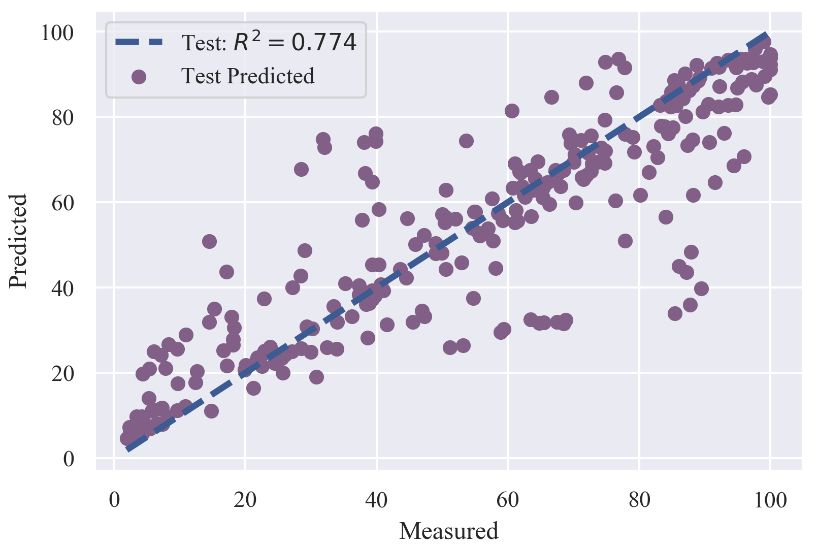
The in vitro dissolution profile of solid dispersion is a key property for its formulation design. Here we established a model to predict the dissolution rate of solid dispersion. It can be used to predict the dissolution rate of drug molecules combined with various polymers within different time periods.
The "maintain supersaturation" (non-precipitation) dissolution profiles were used to establish a regression model.
The drug concentration at 5, 10, 15, 20, 30, 45, and 60 min were chosen to represent the whole dissolution profiles.
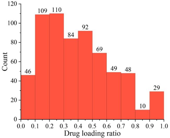
Finally, we got a dataset containing 4214 samples with the 7 time points as a descriptor.
The dataset was split into two parts: training set (3941) and test set (273). The test set was manually picked up
considering the chemical space of both drugs and polymers and included all dissolution profiles of 39 drugs at last.
PyBioMed was used to calculate drug molecular descriptors and MOE software was used to calculate descriptors
of polymers. We tried PLS, RF and LightGBM, finally we got a robust model by using RF.
The best RF model reported a Q2 of 0.892 for 5-fold cross validation and 0.774 for R2 of the test set.
The detailed information was shown as follows.
| Training set: | 3941 |
| Test set: | 273 |
| Q2cv | 0.892 |
| RMSEcv | 10.968 |
| MAEcv | 7.416 |
| R2t | 0.774 |
| RMSEt | 14.195 |
| MAEt | 9.282 |
This platform is consist of 3 main prediction module and 2 kinds of tools. Users can use any one module to realize the corresponding calculation or combine them to evaluate the SD dissolution formulation in a systematic way. Here, we provide some videos to show how to use each module.